Phase 1
Dataset preparation
The German Traffic Sign Recognition Benchmark (GTSRB) dataset was chosen.
What was done
- Dataframe construction
- for every sample, translated its image file into a 3D array (with multiple channels)
EDA
Exploratory Data Analysis was conducted to understand the distribution and variance within the visual data.
What was done
- Class Balance Analysis
- Plotted the number of samples per traffic sign class (0 to 42) using a bar chart to observe potential class imbalances.
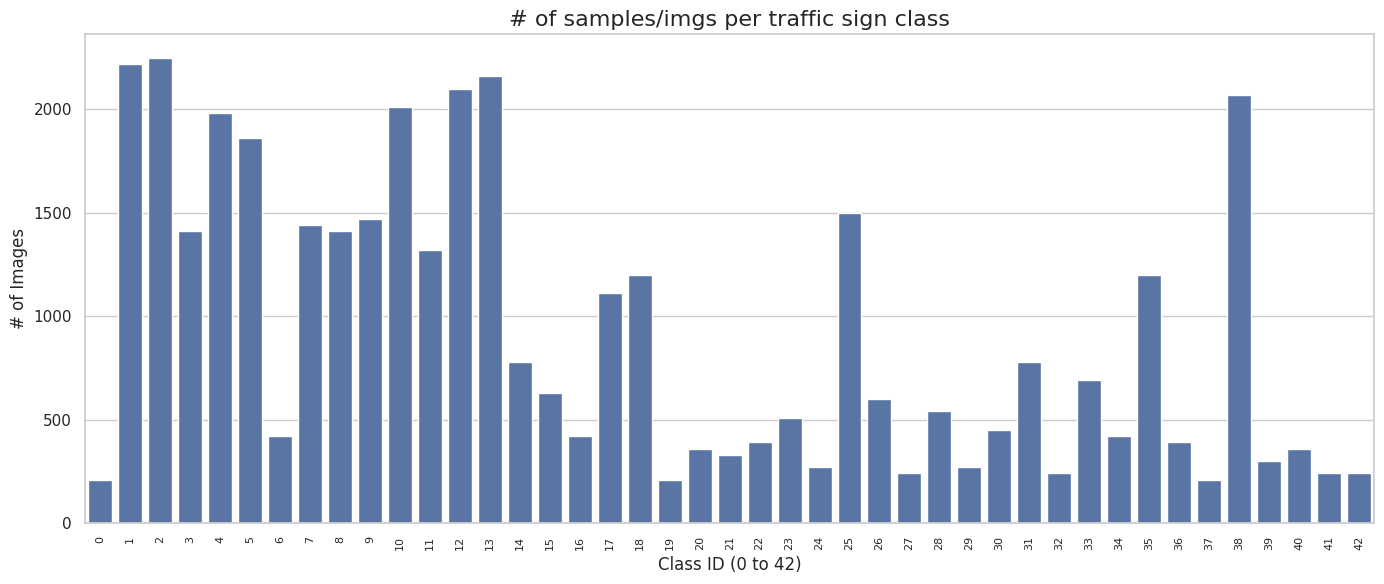
- Plotted the number of samples per traffic sign class (0 to 42) using a bar chart to observe potential class imbalances.
- Raw Image Visualization & Region of Interest (ROI)
- Extracted the bounding box coordinates (
Roi.X1,Roi.Y1,Roi.X2,Roi.Y2) from the dataset to identify the specific region of interest in each image.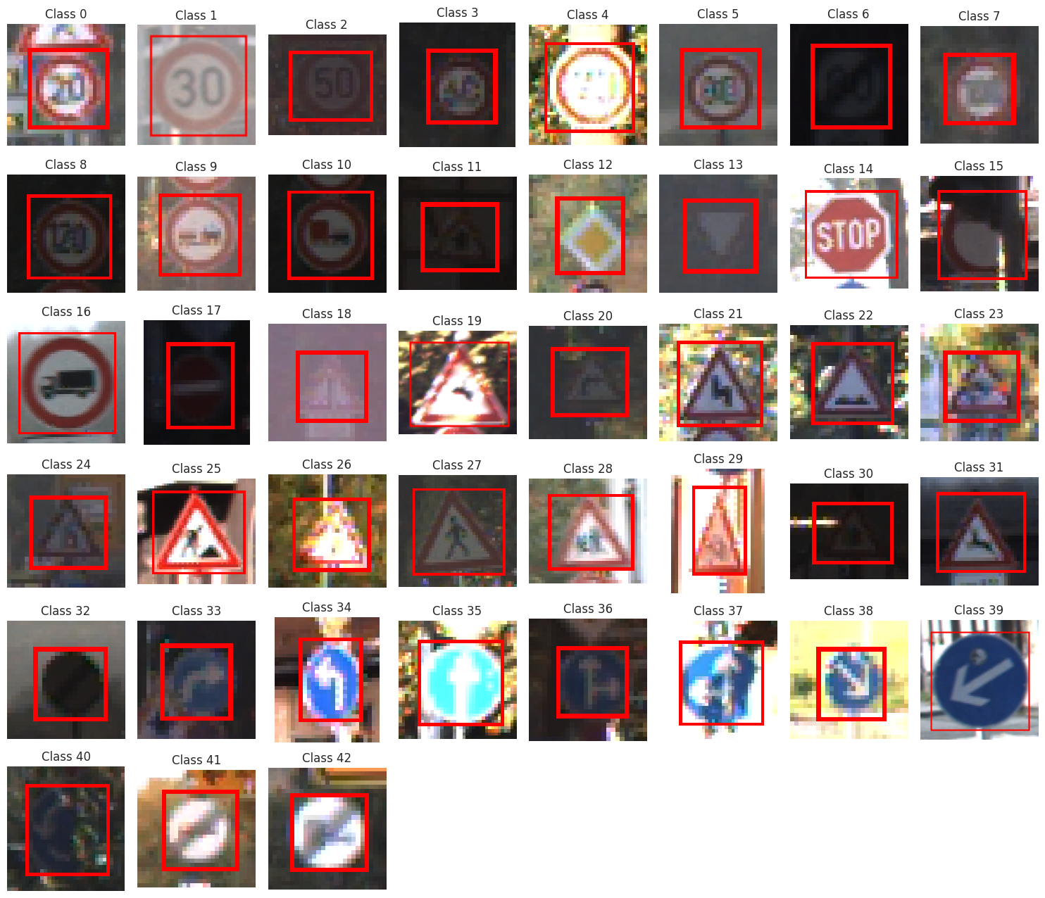
- Extracted the bounding box coordinates (
- Lighting Condition Analysis
- Visualized the distribution of image brightness across classes using a boxplot, showing heavy variances in contrast and lighting.
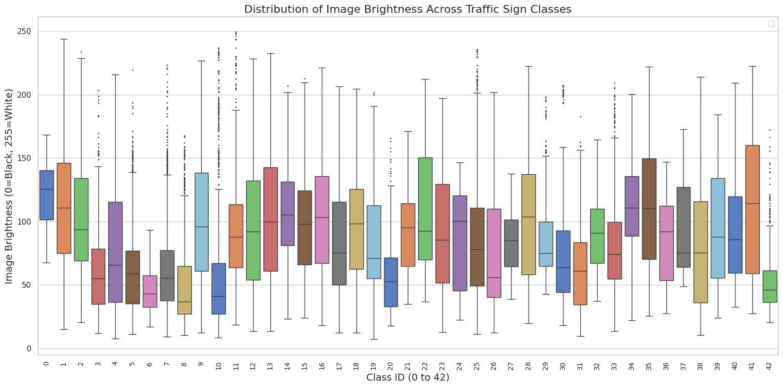
- Visualized the distribution of image brightness across classes using a boxplot, showing heavy variances in contrast and lighting.
Features Preparation
To prepare the dataset for both traditional and deep learning classifiers, it needed some work
What was done
- Cropping and Resizing (for deep learning)
- Cropped each image to its exact ROI bounding box.
- to remove background noise.
- Standardized all cropped images to a fixed resolution.

- Cropped each image to its exact ROI bounding box.
- Flattening
- Flattened the images into a 1D array.
- Scaling (for both)
- Scaled the pixel values using a normalizer.
PCA
Implemented PCA and picked the one to use, using its explained variance plot.
What was done
- Initial PCA transformer
- Initially chose 50 as the # of principal components to keep, but…
- Choosing the one
- its variance plot showed that 30 components were sufficient (they explained 90%).
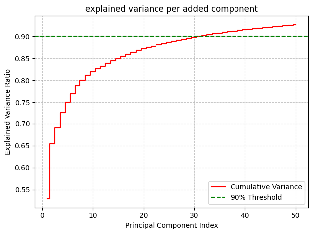
- thus, I switched to one with 30 components.
- its variance plot showed that 30 components were sufficient (they explained 90%).
LDA
Implemented LDA as an alternative for class-aware dimensionality reduction.
What was done
- Maximizing Class Separation
- Applied LDA with 10 components.
- Plotted the cumulative variance to visualize how well the discriminant indices separated the traffic sign classes.

NOTE
- from this point on, the PCA transformed features were used in ML classifiers.
- the # of samples also was reduced to 5000, since ML classifiers don’t use the GPU and take way TOO long to run.
KNN
A K-Nearest Neighbors classifier was implemented from scratch.
What was done
- Grid Search Optimization
- Ran
GridSearchCVtesting . - Discovered that yielded the best parameters.
- Ran
Performance
- Accuracy
- 76.50%
- F1
- 0.7636
- ROC AUC
- 0.8781
Not the worst performance, especially since only a subset of the data was used.
Gaussian Naive Bayes
A Gaussian Naive Bayes classifier was implemented from scratch.
What was done
- Training (Mean & Variance)
- Grouped the training data by class and calculated the mean () and variance () for every feature.
- Added a small epsilon value (
1e-9) to the variance to prevent numerical instability.
- Predicting (Log Posteriors)
- used log-likelihoods.
Performance
- Accuracy
- 18.33%
- F1
- 0.1965
- ROC AUC
- 0.6805
Its performance was really terrible. why?
- gaussian naive bayes assumes that all the features (pixel values) are independent.
- pixels within the same neighborhood are highly dependent.
Ensemble
To improve the stability of the scratch models, an ensemble approach was applied.
What was done
- Bagging
- Wrapped the custom KNN model inside a
BaggingClassifier. - Trained 5 estimators on random subsets of the data (bootstrapping) to reduce variance and output an aggregated prediction.
- Wrapped the custom KNN model inside a
Phase 2
CNN
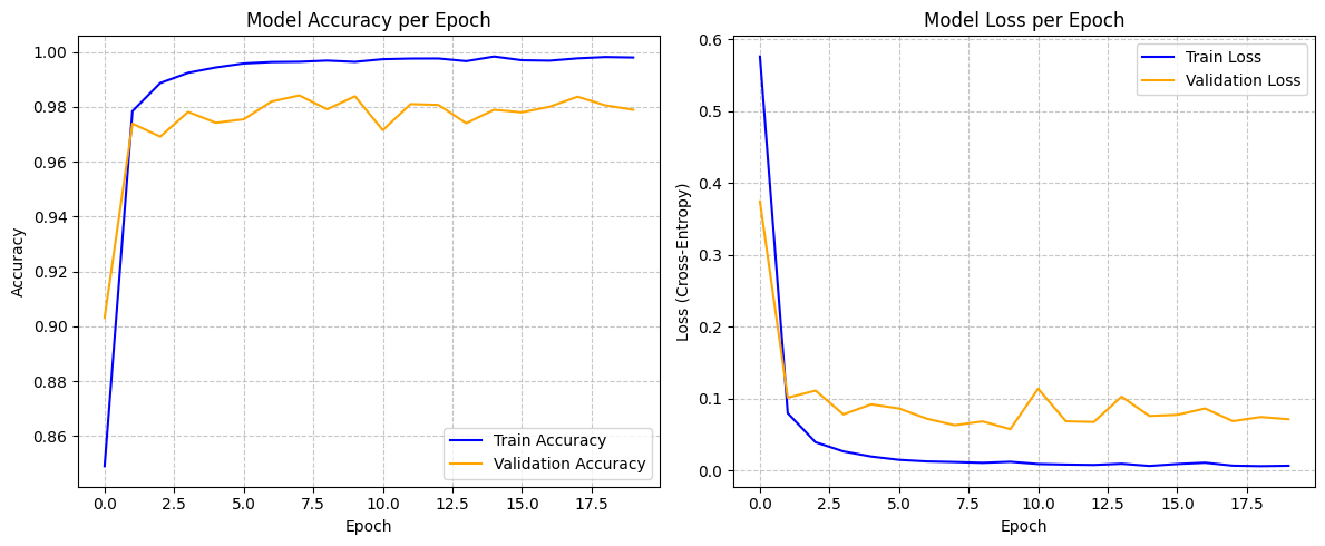
A Convolutional Neural Network (CNN) was implemented from scratch to natively handle the 2D spatial structures within the images.
What was done
-
Architecture Design
- Normalization
- Initially normalized the training pixels with a
Normalizationlayer.
- Initially normalized the training pixels with a
- Level 1 block
- Used
Conv2Dlayers (32 filters). - this extracts the lowest level features.
- Used
- Level 2 block
- Deeper
Conv2Dlayers (64 filters). - this extracts higher-level traffic sign symbols.
- Deeper
- Classification Head
- Flattened the maps into a 512-neuron
Denselayer with severeDropout(0.5)to prevent overfitting, outputting to a 43-class softmax.
- Flattened the maps into a 512-neuron
- used
BatchNormalizationto efficiently normalize features after every block.


- Normalization
Performance
- Accuracy
- 97.85%
- Loss
- 0.0898
- 0.0898
Optimizer Comparison
Optimized the learning rate decay during the CNN’s training phase.
What was done
- Learning Rate Scheduling
- Implemented
ReduceLROnPlateau. - Set to monitor
val_loss, reducing the learning rate by a factor of 0.2 if the loss plateaus for 3 epochs (with a floor of1e-6).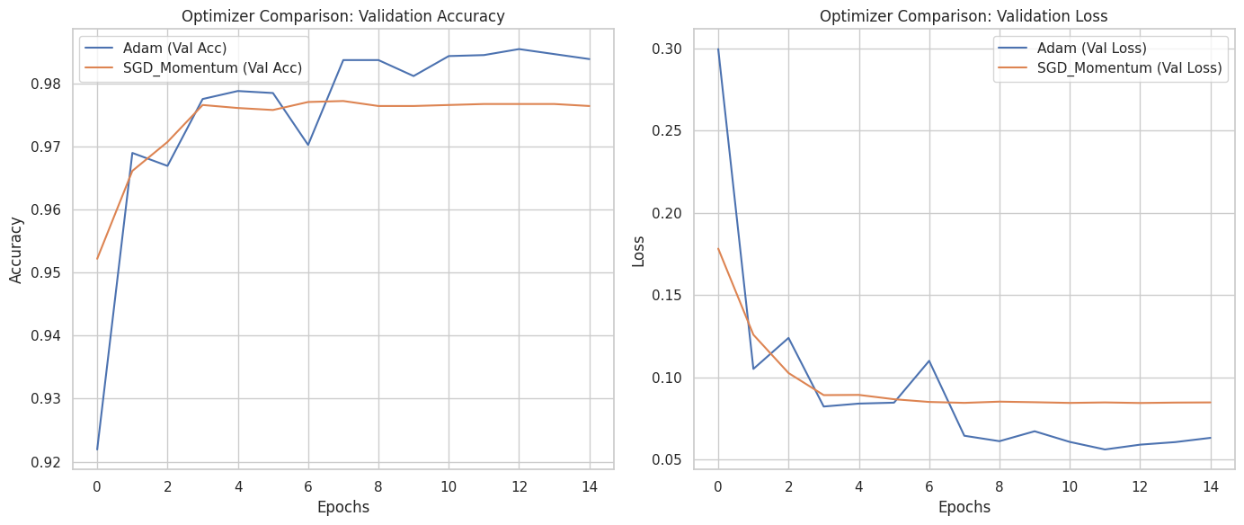
- Implemented
Transfer Learning
Benchmarked the scratch CNN against heavy, pre-trained architectures.
What was done
- Pretrained vs Fine-Tuned
- Loaded
ResNet50andMobileNetV2with ImageNet weights. - Tested both in a purely feature-extraction state (pretrained) and a partially unfrozen state (fine-tuned).
- Loaded
- Performance Conclusion
- Both transfer learning architectures underperformed compared to the custom CNN.
- Hypothesis
- The pretrained models were optimized for large, high-resolution images, whereas the custom CNN was strictly constrained and tailored for the matrices of the GTSRB dataset.
AutoEncoders
An unsupervised Autoencoder pipeline was built to learn visual representations, denoise inputs, and flag anomalous data.
What was done
- Image Enhancement
- Preprocessed the images using CLAHE (Contrast Limited Adaptive Histogram Equalization) to improve local contrast before feeding them to the network.
- Denoising Architecture
- Injected artificial Gaussian noise (
noise_factor = 0.1) into the training images. - Built a bottleneck architecture with Convolutional and MaxPooling downsampling (Encoder) and UpSampling2D (Decoder).
- Trained the model mapping the noisy input directly to the clean target, optimizing via Mean Absolute Error (MAE).
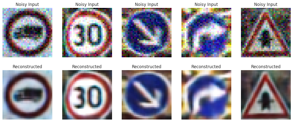
- Injected artificial Gaussian noise (
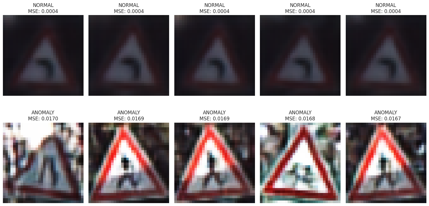
- Anomaly Detection
- Reconstructed the test set and calculated the Mean Squared Error (MSE) of the reconstructions.
- Established a 95th-percentile threshold. Images exceeding this reconstruction error threshold were flagged as “Anomalies.”
- Visualized the “Best” (normal) vs “Worst” (anomalous) reconstructions to verify the system’s filtering logic.